Can GraphCast Predict 10-Day Weather in 1 Minute? How Accurate Is DeepMind's New Forecasting Model? | Yunqi Science Chat

DeepMind and Google have developed GraphCast, a machine learning-based weather simulator that can predict weather up to 10 days out in just 60 seconds — with remarkable accuracy.

1. GraphCast is a graph neural network-based autoregressive model that outperforms the world's most accurate machine learning weather forecasting system (medium-range weather forecasting);

2. GraphCast requires only a single Cloud TPU v4 device to generate 10-day weather forecasts (35GB of data) in 60 seconds, with resolution up to 0.25°;

3. Training on larger, newer, higher-quality data can further improve GraphCast's prediction speed and accuracy.

This edition of "Yunqi Kepu" shares the latest on GraphCast. Enjoy~

Source | WeChat account "AI Era" | Edited by Haokun, Aeneas

➤➤➤ Medium-range weather forecasting has long been a challenge due to massive data volumes. Now, DeepMind and Google's new ML model GraphCast has outperformed existing forecasting models by over 99%.

| Paper: https://arxiv.org/abs/2212.12794

"

Why Medium-Range Weather Forecasting Is So Hard

"Medium-range weather forecasting" typically refers to predicting weather trends 4 to 10 days into the future. Its accuracy is critical for policy-making in agriculture, construction, tourism, and other industries.

To meet this need, the leading European Centre for Medium-Range Weather Forecasts (ECMWF) provides up to four medium-range forecasts daily.

The production process involves two key components, both requiring simulation on large-scale high-performance computing (HPC) clusters:

• Analyzing current and historical data collected from satellites, weather stations, ships, and other sources to predict weather conditions — known as "data assimilation";

• Using numerical weather prediction (NWP) systems to model how weather-related variables will change over time.

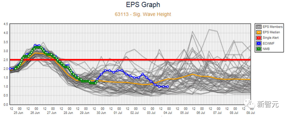
However, as data volumes have grown significantly, NWP models have failed to scale effectively.

In other words, despite vast archives of weather and climate observations, we struggle to directly leverage this data to improve forecast quality.

The conventional approach to improving NWP involves trained experts manually developing better models, algorithms, and approximations — a time-consuming, labor-intensive, and costly process.

By contrast, machine learning-based methods can utilize more and higher-quality available data to improve model accuracy, typically at much lower computational cost.

"

GraphCast

In the paper "GraphCast: Learning Accurate Medium-Range Global Weather Forecasting", DeepMind uses an "encode-process-decode" architecture with graph neural networks (GNNs) to create an autoregressive model.

GraphCast's three-stage simulation process works as follows:

1. Using a GNN with directed edges from grid points to a multi-grid, it maps input data from the raw latitude-longitude grid to learned features on the multi-grid;

2. A deep GNN performs learned message passing on the multi-grid, where long-range edges enable efficient spatial propagation of information;

3. The decoder maps the final multi-grid representation back to the latitude-longitude grid and performs any necessary operations.

Results show that GraphCast outperformed the existing most accurate machine learning weather forecasting model on 99.2% of 252 variables; and exceeded ECMWF's high-resolution forecast (ECMWF HRES Forecast) on 90% of 2,760 variables.

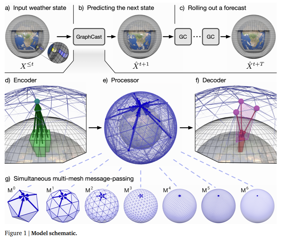
(a) Input weather states are defined on a high-resolution latitude-longitude-pressure level grid.

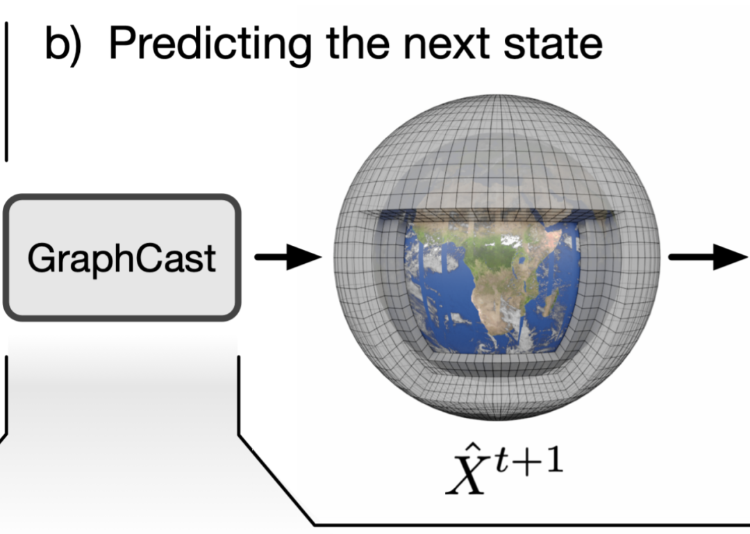
(b) GraphCast predicts the next weather state on a latitude-longitude-pressure level grid.

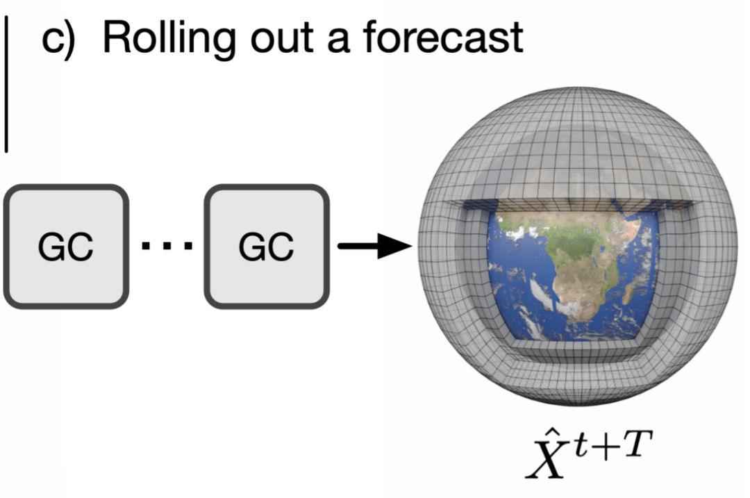
(c) By iteratively applying GraphCast to each previous predicted state, a sequence of states is produced, representing weather at successive lead times.

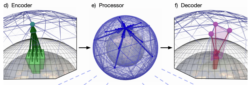
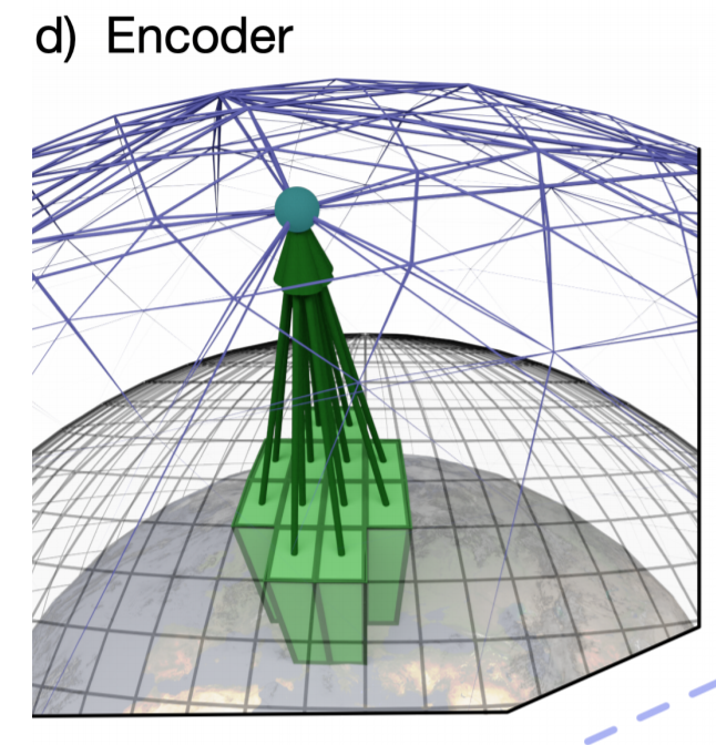
(d) GraphCast's encoder component maps input local regions (green boxes) to nodes on the multi-grid graph.

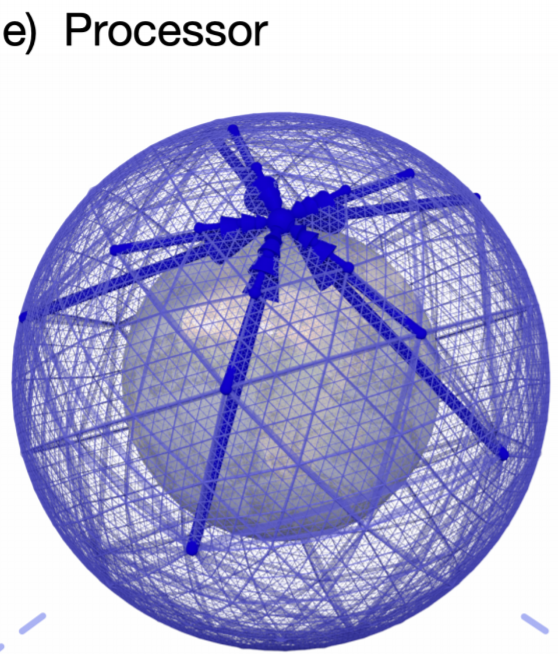
(e) The processor component uses learned message passing to update each multi-grid node.

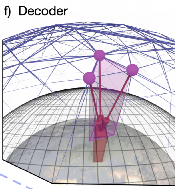
(f) The decoder component maps processed multi-grid features (purple nodes) back to a grid representation.

ERA5 Dataset

GraphCast was trained on a corpus of 39 years (1979–2018) of historical weather data: ECMWF's ERA5 reanalysis dataset.

The model makes 10-day predictions at 6-hour time steps and 0.25° latitude-longitude resolution, covering 5 surface variables and 6 atmospheric variables, each at 37 vertical pressure levels — representing weather states at specific locations and times.

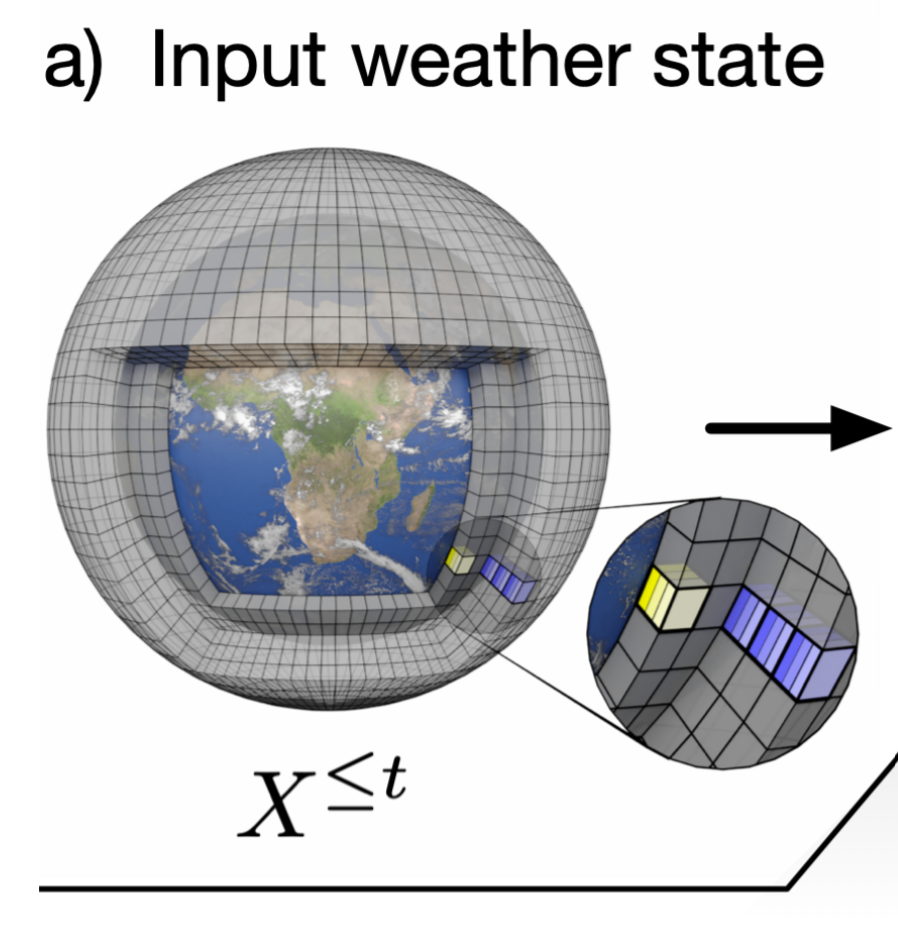
As shown in Figure 1a, researchers represent the weather state at time index t as .

The grid wrapping around Earth corresponds to variables at each latitude, longitude, and pressure level. Surface and atmospheric variables are represented by yellow and blue boxes in the magnified view, respectively.

We refer to the subset of variables corresponding to a specific grid point 𝑖 (1,038,240 total) in as , and each variable 𝑗 among 227 target variables as .

Generating Predictions

GraphCast takes two weather states 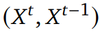as input, corresponding to current time t and previous time t-1, and predicts the weather state at the next time step (as shown in Figure 1b).

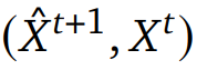
To generate a T-step prediction , GraphCast iteratively applies the equation above in an autoregressive manner, using its own predictions as input to forecast subsequent steps (i.e., for step t+2, input is ; for step t+3, input is ).

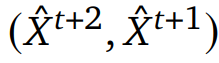Figures 1b and 1c illustrate this process.

Architecture

GraphCast's core architecture uses GNNs in an "encode-process-decode" configuration, as shown in Figures 1d, e, and f.

GNN-based learned simulators are highly effective at learning complex physical dynamics of fluids and other materials because their representation and computational structure resemble finite-element learned solvers.

A key advantage of GNNs is that the input graph structure determines which parts of the representation interact through learned message passing, enabling arbitrary patterns of spatial interaction at any scale.

By contrast, convolutional neural networks (CNNs) are limited to computing interactions within local patches (or, in the case of dilated convolutions, regularly spaced longer ranges).

While Transformers can also perform arbitrary long-range computations, they don't scale well with very large inputs (recall that GraphCast's global input contains over 1 million grid points), because the all-to-all interactions in their computation create prohibitive quadratic memory costs.

Contemporary extensions of Transformers typically sparsify possible interactions to reduce complexity, making them effectively similar to GNNs.

By introducing GraphCast's internal multi-grid representation, researchers leveraged GNNs' ability to model arbitrarily sparse interaction patterns.

It has uniform spatial resolution globally and enables long-range interactions within a small number of message passing steps.

To construct a multi-grid, a regular icosahedron (12 nodes, 20 faces) is iteratively refined 6 times, yielding a hierarchy of icosahedral grids with 40,962 nodes and 81,920 faces at the finest resolution.

Since coarse-grid nodes are subsets of fine-grid nodes, researchers can overlay edges from all levels of the grid hierarchy onto the finest-resolution grid.

This produces a multi-scale mesh set where coarse edges bridge long distances across scales, and fine edges capture local interactions.

Figure 1g shows each individual refinement level, while Figure 1e shows the complete multi-grid.

Using a GNN with directed edges from grid points to multi-grid, GraphCast's encoder (Figure 1d) first maps input data from the raw latitude-longitude grid to learned features on the multi-grid.

Then, the processor (Figure 1e) uses a 16-layer deep GNN for learned message passing on the multi-grid, where long-range edges enable efficient spatial propagation of information.

Finally, the decoder (Figure 1f) uses a GNN with directed edges to map the final multi-grid representation back to the latitude-longitude grid, combining this grid representation Ŷᵗ⁺ᵏ with the input state X̂ᵗ⁺ᵏ to form the output prediction, X̂ᵗ⁺ᵏ⁺¹ = X̂ᵗ⁺ᵏ + Ŷᵗ⁺ᵏ.

Training Process

GraphCast was trained to minimize the objective function against ERA5 targets over 12 prediction steps (3 days) using gradient descent.

The objective function is as follows —

Researchers trained GraphCast for approximately 3 weeks on 32 Cloud TPU v4 devices using batch-parallel techniques.

To reduce memory footprint, they also employed sophisticated gradient checkpointing strategies and low-precision numerics.

Results

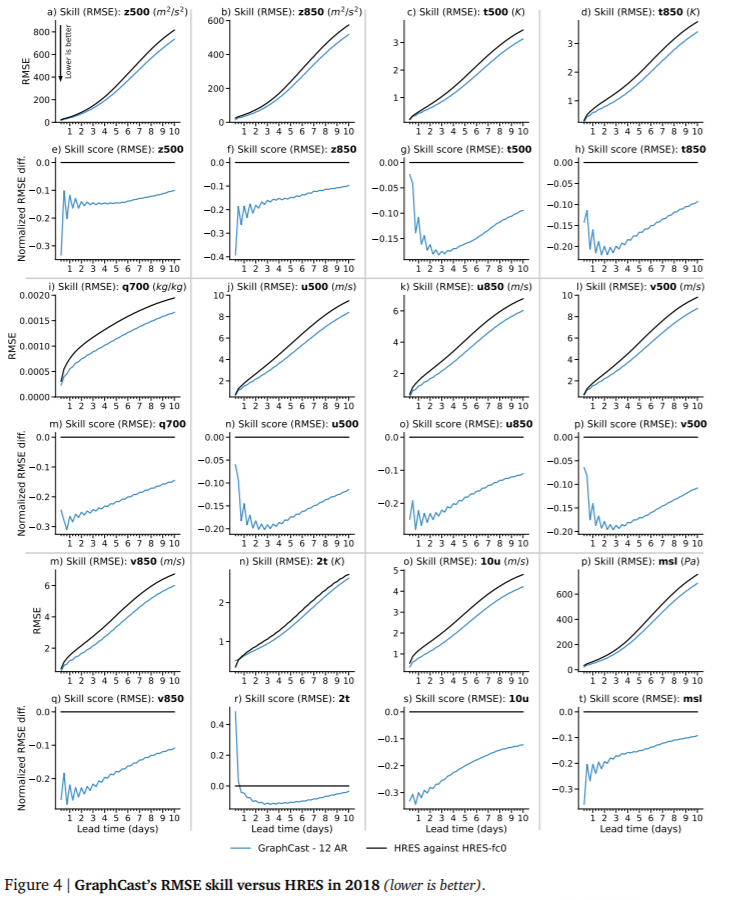
Results show that GraphCast comprehensively surpassed HRES weather forecasting technology in 10-day forecasts at 0.25° resolution.

As shown in Figure 4, GraphCast (blue line) significantly outperforms HRES (black line) across 10 major surface and atmospheric variables.

Furthermore, regional analysis indicates these results are consistent across the globe.

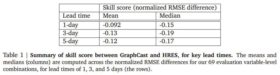
Based on evaluation results, GraphCast outperformed HRES on 90.0% of 2,760 variable, level, and lead-time combinations (4 surface variables plus 5 atmospheric variables × 13 levels, over 10 days at 4 steps per day).

Researchers note that HRES tends to outperform GraphCast at upper atmospheric levels, particularly at the 50 hPa pressure level, which is unsurprising given that the total training loss weight applied to pressure levels at 50 hPa or below accounts for only 0.66% of the total loss weight across all variables and levels.

When excluding the 50 hPa level, GraphCast outperforms HRES on 96.6% of 2,240 targets; when excluding both 50 and 100 hPa levels, this rises to 99.2% of 1,720 targets.

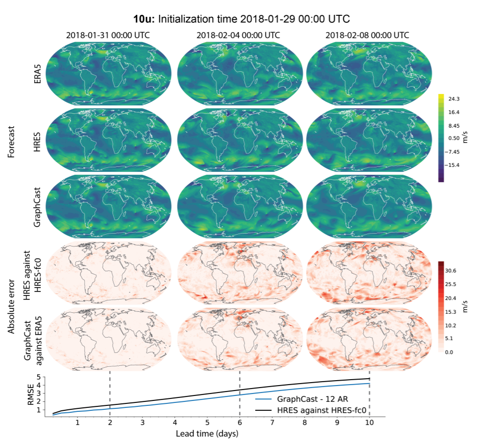
10u true and predicted weather. Row 1 shows ERA5, Row 2 shows HRES, Row 3 shows GraphCast, Rows 4 and 5 show absolute error maps between HRES and HRES-fc0, and between GraphCast and ERA5. Bottom plots show RMSE levels for HRES and GraphCast.

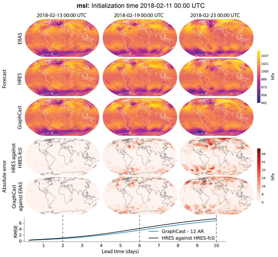
msl true and predicted weather states

Impact of Autoregressive Training on Predictions

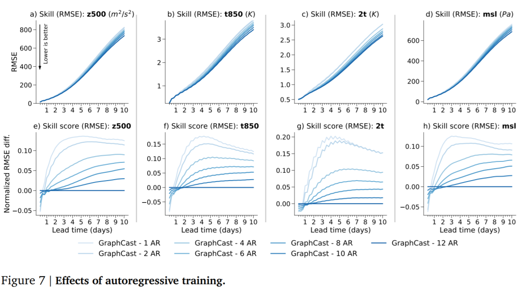
When trained with fewer autoregressive steps, models perform better at shorter lead times but worse at longer lead times.

As autoregressive steps increase, performance degrades at shorter lead times but improves at longer lead times.

GraphCast vs. Top ML Prediction Models

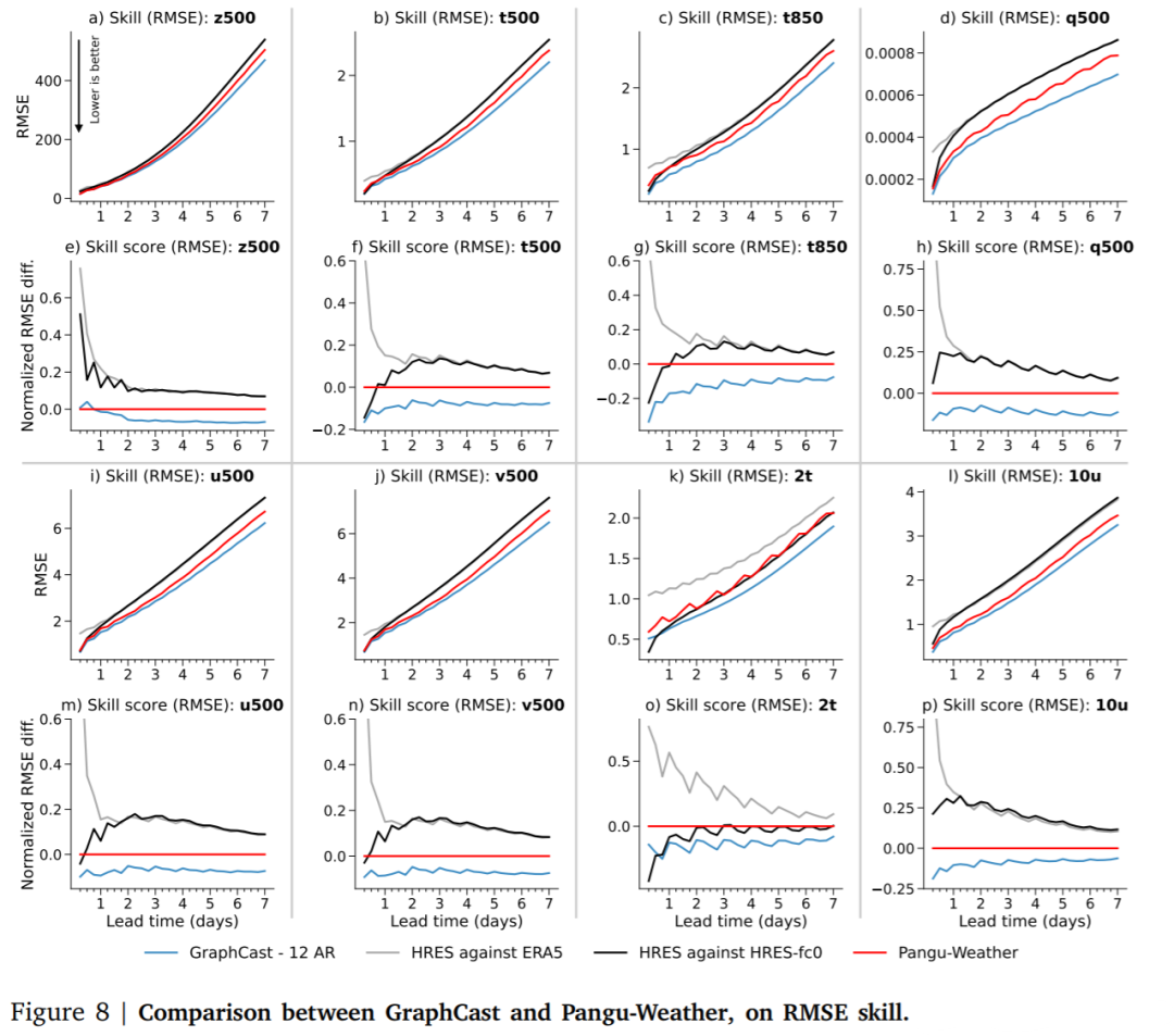
Currently, ViT-based Pangu-Weather represents the state of the art in ML-based weather forecasting, with a computational pattern similar to GNNs.

Comparison results between GraphCast and Pangu-Weather are shown in Figure 8. Rows 1 and 3 show absolute RMSE for GraphCast (blue), Pangu-Weather (red), HRES evaluated against HRES-fc0 (black), and HRES evaluated against ERA5; Rows 2 and 4 show normalized RMSE differences between models relative to Pangu-Weather.

Summary

The GraphCast model outperformed ECMWF's HRES — currently the most accurate deterministic system — in 10-day forecasts at 6-hour steps and 0.25° latitude-longitude resolution.

Evaluated across 2,760 combinations of variables, pressure levels, and lead times, GraphCast achieved lower RMSE than HRES on 90.0% of metrics.

When excluding upper atmospheric fields at 100 hPa and above, GraphCast outperformed HRES on 99.2% of 1,760 targets.

Additionally, GraphCast exceeded the previous best ML baseline — Pangu-Weather — on 99.2% of 252 targets.

A key innovation of GraphCast is its novel "multi-grid" representation, enabling it to capture much longer-range spatial interactions than traditional NWP methods, thereby supporting coarser native time steps.

This is part of why GraphCast can generate accurate 10-day weather forecasts in 60 seconds at 6-hour intervals on a single Cloud TPU v4 device.